· 6 min read
Abid Arcot

In the realm of digital circuits, implementing mathematical functions efficiently is paramount for various applications, from signal processing to machine learning. In this technical exploration, we delve into the optimization of hardware implementations for one such crucial function: the exponential function (ex)(e^x).

Introduction

The task at hand involves implementing the exponential function for 16-bit fixed-point input values. While numerous methods exist for hardware realization, we opted for a Taylor expansion-based approach due to its simplicity and effectiveness. The 5th Taylor polynomial approximation serves as our foundation, providing a balance between accuracy and computational complexity.

Taylor Expansion of the Exponential Function:

The Taylor expansion of the exponential function exe^x is given by:

ex=n=0xnn!=1+x+x22!+x33!+x44!+x55!+ e^x = \sum_{n=0}^{\infty} \frac{x^n}{n!} = 1 + x + \frac{x^2}{2!} + \frac{x^3}{3!} + \frac{x^4}{4!} + \frac{x^5}{5!} + \ldots

Baseline Implementation

Our journey begins with the baseline implementation, a fundamental circuit computed through Verilog. This circuit, rooted in the 5th Taylor polynomial, forms the cornerstone for subsequent optimizations. With a clear understanding of its functionality and performance metrics, we embark on the quest for enhancement.

Circuit Diagram:

Baseline Circuit Diagram

Figure 1: The baseline circuit for computing the 5th5^{th} Taylor polynomial approximating exe^x. Where y=((((a5x+a4)x+a3)x+a2)x+a1)x+a0,a0=1,a1=1,a2=12,a3=16,a4=124,a5=1120 y = ((((a5x + a4)x + a3)x + a2)x + a1)x + a0, a_0 = 1, a_1 = 1, a_2 = \frac{1}{2}, a_3 = \frac{1}{6}, a_4 = \frac{1}{24}, a_5 = \frac{1}{120}

The Verilog code for the baseline implementation computes the 5th Taylor polynomial approximation of exe^x. It takes 16-bit fixed-point input values in Q2.14 format and produces 32-bit fixed-point outputs in Q7.25 format. The circuit consists of multipliers and adders arranged in a sequential manner to compute the polynomial terms and accumulate the result. Source code can be found here.

Pipeline Optimization

The first stop on our optimization journey leads us to the realm of pipelining. By introducing pipelines for multipliers and adders, we aim to enhance throughput and mitigate critical path delays. Leveraging registers strategically, we achieve a pipeline latency of 10 cycles, ensuring a steady stream of outputs with minimal overhead. Source code can be found here.

Pipeline Block Diagram:

Pipeline Block Diagram

Figure 2: The pipeline circuit, where purple blocks are registers.

Thorough functional verification validates the efficacy of our pipelined design. Through waveform analysis and meticulous testing, we confirm the expected pipeline latency and ascertain the accuracy of our outputs.

Shared Hardware Design

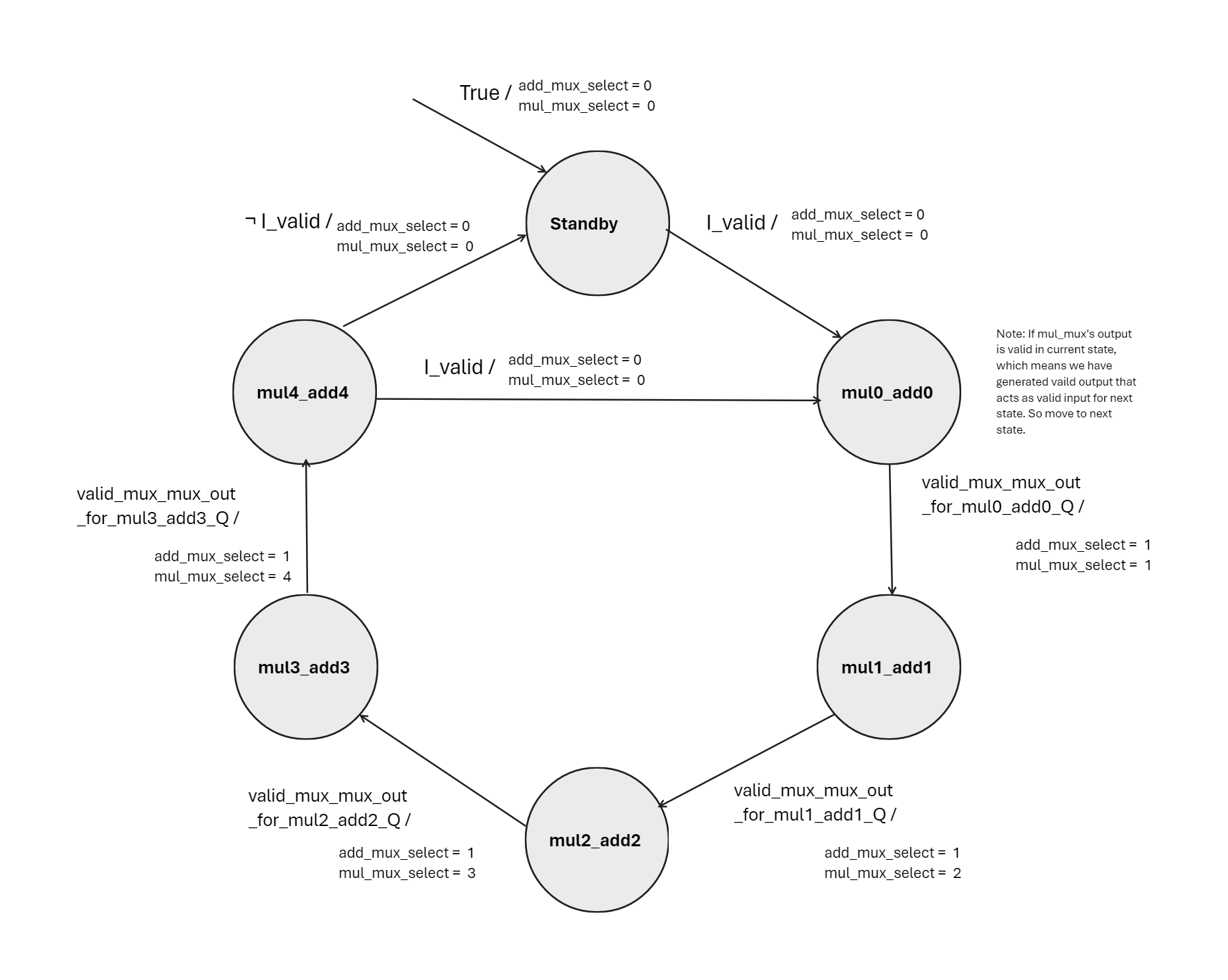
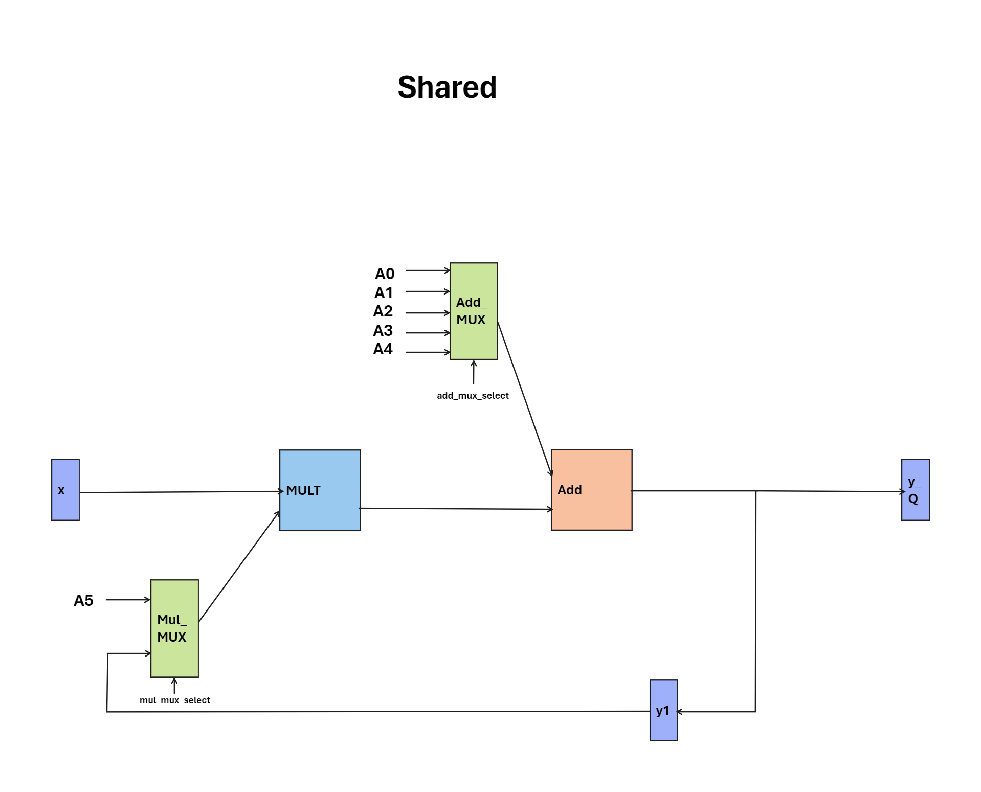
In the shared hardware design, through the harmonious coordination of multipliers and adders orchestrated by a finite state machine (FSM), we aim to achieve optimal efficiency while maintaining high performance standards. Every input initiates a meticulously synchronized series of actions, resulting in outputs produced at regular intervals of 5 cycles. Source code can be found here.

Shared Hardware and FSM Diagram:
Shared Hardware Design

Figure 3: The shared circuit, where purple blocks are registers.

FSM

Figure 4: FSM for shared circuit.

Comparative Analysis

With our optimized designs in hand, we conduct a comprehensive comparative analysis to gauge their efficacy. From resource utilization to operating frequency and throughput, each design undergoes meticulous scrutiny. The pipeline emerges as the champion in throughput, leveraging its enhanced frequency of operation to deliver unparalleled performance.

Exact vs. Approximated Exponential Function

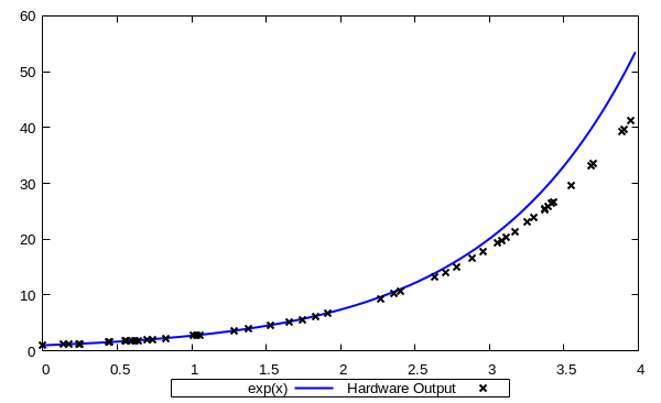
As we are reimplementing same circuit for baseline, pipeline, and shared, we achieved same accuracy
Graph

Figure 5: Exact vs. Approximated Exponential Function.

Efficiency Metrics:

We calculate efficiency metrics for each design based on resource utilization, operating frequency, throughput, and dynamic power consumption. It's important to note that these metrics are calculated assuming the whole device is filled with maximum replications for a given circuit design, where the maximum DSP slices available are 1518.

MetricBaseline CircuitPipelined CircuitShared HW Circuit
Resources for one circuit36 ALMs + 6 DSPs92 ALMs + 4 DSPs34 ALMs + 2 DSPs
Operating frequency47.7 MHz213.35 MHz146.13 MHz
Critical pathDSP mult-add + 2x DSP mult + LE-based adder + 6x DSP mult + LE-based adderMult1 (2 ALMs) + Addr1 (1 ALM) + Mult2 & y4 (1 DSP)State (1 FF) + multiplier’s mux (1 ALM) + Mult (2 DSPs) + Addr (1 ALM) + y_Q (1 FF)
Cycles per valid output1pipeline latency = 10, 1 cycle for every output after first output.5
Max. # of copies/device253 (i.e. 1518 DSPs/6)379 (i.e. 1518 DSPs/4)759 (i.e. 1518 DSPs/2)
Max. Throughput for a full device (computations/s)12,068.1 Million computations/s (i.e. 253 * 47.7 MHz)80,859.65 Million computations/s (i.e. 379 * 213.35 MHz)22,182.534 Million computations/s (i.e. 759 * 146.13 MHz / 5)
Dynamic power of one circuit21.41 mW18.28 mW7.76 mW
Max. throughput/Watt for a full device2.23 billion computations/Watt (i.e. Max. Throughput/(21.41mW * 253 ))11.67 billion computations/Watt (i.e. Max. Throughput/(18.28 mW * 379 ))3.76 billion computations/Watt (i.e. Max. Throughput/(7.76 mW * 759))

Toggle Rate Analysis:

We also analyze the toggle rates for each design, which indicates how often signals change in the circuit.

Circuit DesignToggle Rate (Million Transitions/s)
Baseline134.086
Pipelined129.790
Shared HW140.558

Conclusion

In conclusion, our exploration into optimizing hardware implementations of the exponential function has yielded significant insights and effective strategies. We've observed that implementing a few terms of Taylor’s expansion leads to some level of inaccuracy, which can be mitigated by incorporating more terms for enhanced precision. Furthermore, while clipping the most significant and least significant bits during multiplication to fit the Q7.25 format introduces some loss of accuracy, widening inputs and outputs to achieve the desired precision before formatting to Q7.25 in the final stage can counteract this effect.

In terms of circuit efficiency, our analysis of toggle rates reveals that the pipelined design boasts the lowest toggle rate. Despite having larger circuitry than the other two designs, its lower toggle rate underscores its greater efficiency.

The pipelined architecture stands out for its ability to achieve the highest throughput, owing to the benefits of pipelining that allow for a higher frequency of operation and output generation. Compared to the baseline and shared designs, the pipelined approach excels in both frequency of operation and frequency of output generation.

· 7 min read
Abid Arcot

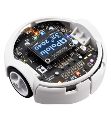
This blog aims to guide you through the process of programming a Pololu robot to execute a specific set of actions: ascending a ramp, recognizing the summit, changing direction, and safely descending the ramp without the risk of falling off. We will delve into best practices for designing an embedded system, breaking down the process into modeling, designing, and analyzing.

Throughout this journey, we'll navigate the intricacies of implementing line sensing, feedback control, and accelerometer integration to ensure our robot successfully ascends a ramp, executes a turn at the top, and descends without veering off the edge.

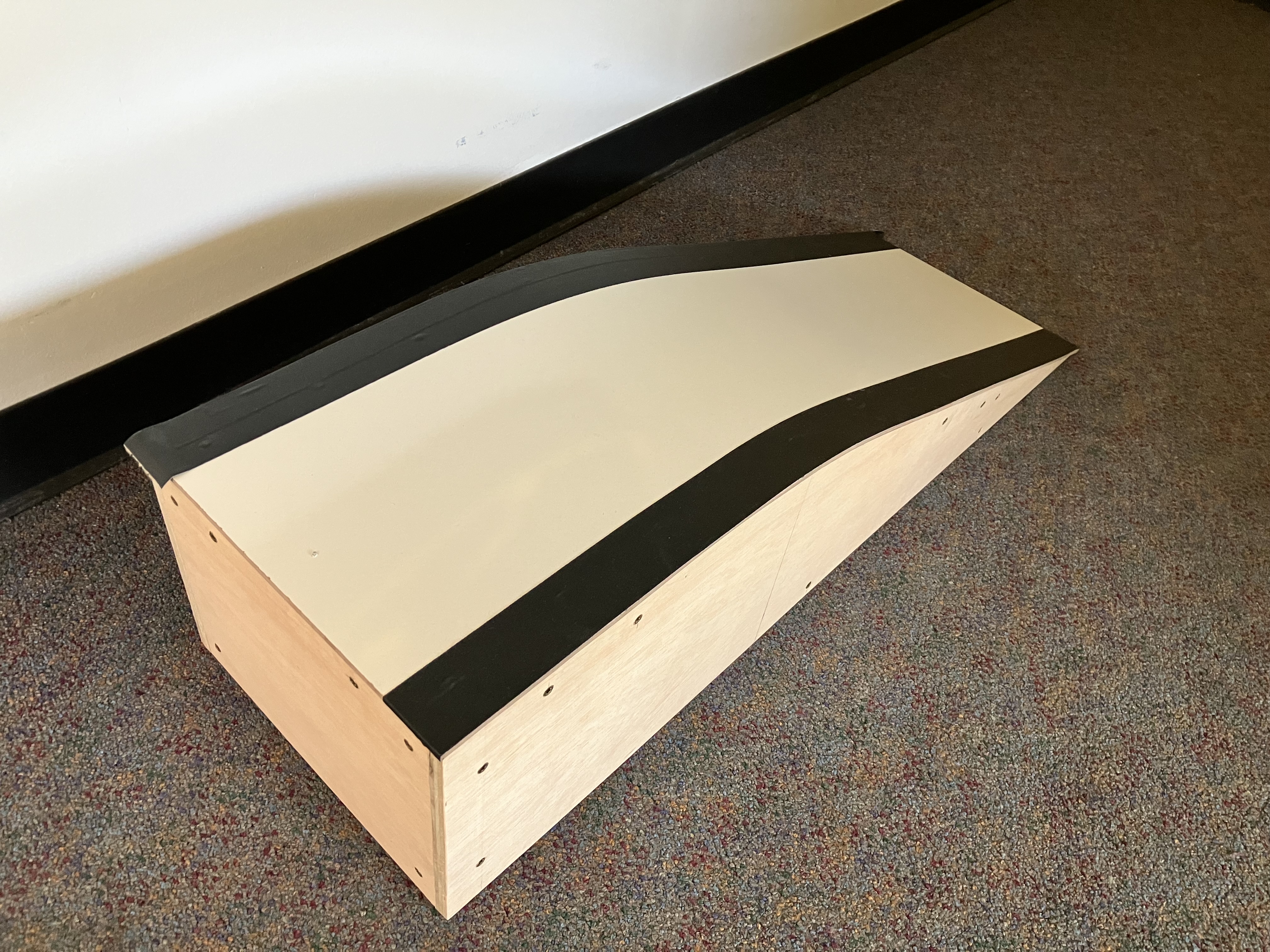
Ramp

Background

For this project, we will utilize Lingua Franca, the first reactor-oriented coordination language. It allows you to specify reactive components and compose them. Lingua Franca's semantics eliminate race conditions by construction and provide a sophisticated model of time, including a clear and precise notion of simultaneity. The blog will explain the concepts sufficiently for you to comprehend the program, even if you're not familiar with the language.

To kickstart our project, we'll fork lf-3pi-template, which comes with pico-sdk, facilitating a quick start.

Understanding the Task at Hand

Our primary goal is to program the Pololu robot to perform a specific sequence: climb a ramp, detect the summit, turn around, and descend without falling off the edge. Key elements for this challenge include a ramp with a 15-degree slope, a flat turning surface at the top, a light-colored surface, and dark-colored edges for the robot to detect and avoid.

Ramp

Modeling

Let's initiate our project by modeling it with a finite-state machine and outlining the sensors we'll use.

Sensors Utilized

Line Sensors

For detecting edges and preventing the robot from falling off the wedge. Additionally, the accelerometer will provide roll, yaw, and pitch values, while the gyroscope calculates the angular velocity for precise turns.

Encoders

Encoders play a crucial role in sustaining a consistent speed during both ascents and descents on the hill, effectively powering the wheels in accordance with the terrain.

Accelerometer

Implement feedback control to adjust individual wheel speed periodically, maintaining a near-zero roll measurement. We will leverage the Motors With Feedback reactor to compensate for roll-induced variations in motor power.

Gyroscope

Utilize the gyroscope to calculate angular displacement for accurate turning of the bot.

(Note: For more details about the implementation of the program for sensors, refer to the src directory)

Finite State Machine

Finite State Machine

Our journey begins in a calibrating state, where we set the line sensor threshold. After a 5-second calibration, we transition to the driving state. Subsequently, the robot defaults to moving forward.

While moving forward, the robot may encounter the dark line or reach the end of the wedge. Upon detection, the robot saves the data, tracks back a few centimeters, and enters the LineDetect state. Decisions in this state are based on the saved data, leading to a 20-degree turn in the opposite direction of the detected line or a 180-degree turn if the wedge's end is detected.

Preparing for the Climb

Before delving into the implementation, it's crucial to outline the key requirements for our robot program:

  • Ascend and descend a ramp with a 15-degree slope.
  • Detect dark-colored edges of the ramp using line sensors.
  • Implement feedback motor control using accelerometer and encoders to adjust wheel speeds based on roll and encoder readings.
  • Perfom precise turns using gyroscope measurements.

Designing/Implementation

my-3pi/src/HillClimbSolution.lf
target C {
platform: {
name: "rp2040",
board: "pololu_3pi_2040_robot"
},
threading: false,
}

import Display from "lib/Display.lf"
import GyroAngle from "lib/IMU.lf"
import LineSensor from "HillLineDetectSolution.lf"
import Tilt from "lib/Tilt.lf"
import Encoders from "lib/Encoders.lf"
import MotorsWithFeedback from "lib/MotorsWithFeedback.lf";


reactor Robot {
output notify:string // Notify of mode change.
state turn_angle:int
state turn_direction:int //+1 for left direciton, -1 for right direction
state lineOnLeft:bool
state lineOnCenter:bool
state lineOnRight:bool
state takenUTurn:bool=false


lineSensor = new LineSensor()
motors = new MotorsWithFeedback();
encoder = new Encoders();

encoder.right -> motors.right;
encoder.left -> motors.left;

tilt = new Tilt()
timer t(0, 10 ms)
timer t2(0, 50 ms)

reaction(startup) -> notify {=
lf_set(notify, "INIT:CALIBRATING");
=}

reaction(t) -> encoder.trigger {=
lf_set(encoder.trigger, true);
=}

initial mode CALIBRATING
{
reaction(lineSensor.left, lineSensor.center, lineSensor.right) -> reset(DRIVING), notify {=
lf_set_mode(DRIVING);
lf_set(notify, "DRIVING");
=}
}

mode DRIVING {

reaction(reset) -> motors.left_speed, motors.right_speed {=
lf_set(motors.left_speed, 0.2); //0.2 m/s
lf_set(motors.right_speed, 0.2);
=}

reaction(t2) -> tilt.trigger{=
lf_set(tilt.trigger, true);
=}

reaction(tilt.x, tilt.y) -> motors.left_speed, motors.right_speed, reset(TURN), notify {=

if(tilt.x->value <= 0 && !self->takenUTurn)//considering we have reached the top, then perfom U-turn
{
self->turn_angle = 180;
self->turn_direction = 1;//direction doesn't matter
self->takenUTurn = true;
lf_set_mode(TURN);
lf_set(notify, "TURN");
}

lf_set(motors.left_speed, 0.2 * (1.0 - 0.05 * tilt.y->value * ((tilt.x->value >= 0) ? 1.0 : -1.0)));
lf_set(motors.right_speed, 0.2 * (1.0 + 0.05 * tilt.y->value * ((tilt.x->value >= 0) ? 1.0 : -1.0)));

=}

reaction(lineSensor.left, lineSensor.center, lineSensor.right) -> reset(LineDetect), notify {=

self->lineOnLeft = lineSensor.left->value;
self->lineOnCenter = lineSensor.center->value;
self->lineOnRight = lineSensor.right->value;

if(self->lineOnLeft|| self->lineOnCenter || self->lineOnCenter)
{
lf_set_mode(LineDetect);
lf_set(notify, "LineDetect");
}
=}
}

mode LineDetect {
logical action turn

reaction(reset) -> motors.left_speed, motors.right_speed, turn, reset(DRIVING), notify {=

lf_set(motors.left_speed, -0.2);
lf_set(motors.right_speed, -0.2);

if(self->lineOnCenter)
{
self->turn_angle = 180;
self->turn_direction = 1;//direction doesn't matter

}
else if(self->lineOnLeft)
{
self->turn_angle = 20;
self->turn_direction = -1; //right
}
else if (self->lineOnRight)
{
self->turn_angle = 20;
self->turn_direction = 1; //right
}
else
{
//no line detected
lf_set_mode(DRIVING);
lf_set(notify, "DRIVING");
}

lf_schedule(turn, SEC(0.4));
=}

reaction(turn) -> reset(TURN), notify{=
lf_set_mode(TURN);
lf_set(notify, "TURN");
=}

}

mode TURN {
gyro = new GyroAngle()

reaction(reset) -> motors.left_speed, motors.right_speed {=
lf_set(motors.left_speed, self->turn_direction * -0.2);
lf_set(motors.right_speed,self->turn_direction * 0.2);
=}

reaction(t) -> gyro.trigger {=
lf_set(gyro.trigger, true);
=}

reaction(gyro.z) -> reset(DRIVING), notify{=
if(abs(gyro.z->value) > self->turn_angle)
{ lf_set_mode(DRIVING);
lf_set(notify, "DRIVING");
}
=}
}


}

main reactor {
robot = new Robot()
display = new Display()
robot.notify -> display.line0;
}

The primary component in the above Lingua Franca program is a reactor, functioning like an object to some extent. The reactor can have multiple states, and it provides mechanisms to transition between states based on time or physical/logical actions. It also has interfaces to input and output the data.

Here, in the program, we have two reactors:

  1. Robot
  2. Display

A Robot reactor has a total of 4 states:

  1. CALIBRATING
  2. DRIVING
  3. LINEDETECT
  4. TURN

The Robot reactor operates exclusively in one of its states at any given time. According to the design, the robot defaults to the CALIBRATING state and then shifts to DRIVING after completing the calibration process. The robot remains in the DRIVING state until it encounters obstacles. Upon detecting obstacles, it retraces a few centimeters, transitioning to the LINEDETECT state. In the LINEDETECT state, a decision is made to navigate around the obstacle. After deciding, it proceeds to the TURN state, determining the number of degrees to turn (let's say x degrees) and the direction (clockwise/anti-clockwise) based on information from LINEDETECT during exit.

Once the TURN state executes actions in line with the decision from LINEDETECT, control shifts back to the DRIVING state, with its default behavior of moving forward. Following the initial CALIBRATING state, the robot continually cycles through the DRIVING, LINEDETECT, TURN states to fulfill its designated task.

Finally, the Display reactor receives input from the Robot reactor to showcase obstacle detection, indicating positions such as left, right, and middle.

Analysis

The robot effectively accomplishes its assigned mission, skillfully steering clear of the dark-colored edges. Moreover, the feedback control adeptly mitigates variations in roll, ensuring a consistent speed both uphill and downhill. Once aligned with the ramp, the robot seamlessly follows a straight path, courtesy of the precise adjustments made by the feedback control system. In instances where the robot starts its task atop the dark-colored edges, it promptly detects the situation and makes informed decisions to evade potential issues.

Conclusion

This project seamlessly combines sensor integration, feedback control, and real-world navigation, offering valuable insights into the intricate challenges of robotics and a practical way to apply the concepts learned from embedded systems courses, including Designing, Modeling, and Analysis. Source code can be found at Github. Stay tuned for more exciting technical explorations in our upcoming blogs!

References

· 9 min read
Abid Arcot

Background: Fully Homomorphic Encryption Unveiled

Before we embark on our comparative analysis of the SEAL and OpenFHE libraries, let's unveil the revolutionary concept of Fully Homomorphic Encryption (FHE). In the realm of cryptography, FHE stands as a beacon of innovation, allowing computations on encrypted data without the need for decryption.

Traditional encryption methods ensure the confidentiality of sensitive information during transmission or storage. However, they often hinder the ability to perform computations on this encrypted data without decrypting it first. FHE, on the other hand, transcends these limitations by enabling operations directly on encrypted data, preserving its confidentiality throughout the computational process.

Introduction

In this technical blog, we delve into the world of FHE and conduct a comparative analysis of two leading open-source libraries: Microsoft SEAL and OpenFHE. Our exploration focuses on the implementation of two widely-used FHE schemes, Brakerski-Gentry-Vaikuntanathan (BGV) and Brakerski/Fan-Vercauteren.

Understanding OpenFHE and SEAL

OpenFHE: A Glimpse into Versatility

OpenFHE, powered by Duality Technologies, emerges as a versatile open-source homomorphic encryption library. Its popularity stems from its support for a diverse range of FHE schemes, including BFV, BGV, CKKS, FHEW, and TFHE. Additionally, OpenFHE incorporates multiparty extensions for threshold FHE and proxy re-encryption, providing a comprehensive toolkit for various cryptographic applications.

Explore OpenFHE: OpenFHE GitHub Repository

To download OpenFHE binaries, visit the OpenFHE GitHub Releases section.

SEAL: Harnessing Microsoft's Expertise

SEAL, an open-source library developed by Microsoft, is designed to implement the most popular FHE schemes in use today: BGV, BFV, and CKKS. Leveraging Microsoft's expertise in cryptography, SEAL offers a robust platform for secure computations over encrypted data.

Explore SEAL: SEAL GitHub Repository

To download SEAL binaries, visit the SEAL GitHub Releases section.

Homomorphic Operations Data and Analysis

For our comparative analysis, we leverage the resources available in the GitHub repository. The repository contains C programs and binaries, facilitating a more detailed and resourceful exploration.

The provided binaries include:

  1. SEAL BGV
  2. SEAL BFV
  3. OpenFHE BGV
  4. OpenFHE BFV

Each binary executes homomorphic addition and multiplication operations on encrypted data, producing runtime and result outputs. These binaries serve as the foundation for our exploration into the efficiency and performance of FHE schemes.

Data Generation and Analysis

To initiate our analysis, we generate at least ten unique combinations of inputs for both multiplication and addition operations, taken average over ten iterations. The resulting tables showcase the runtimes of these operations for each scheme within the SEAL and OpenFHE libraries.

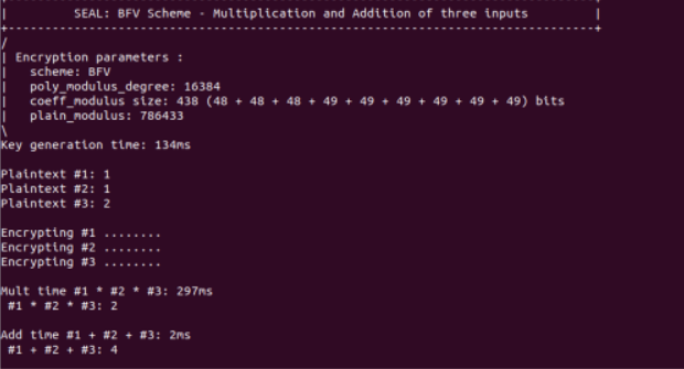
Pre-compiled binaries for the above libraries are provided at GitHub repository. To build you own binaries refer appendix. One can runs the binaries as follows.

./openFHE_BFV 1 1 2

example-img

Sample output when running the provided binary

Multiplication:

Input1Input2Input3OpenFHE_BFVOpenFHE_BGVSEAL_BFVSEAL_BGV
123522611843
456542611547
789552811844
101112562912146
131415562612444
161718582812050
192021572811448
222324522812046
252627552812145
282930562812045

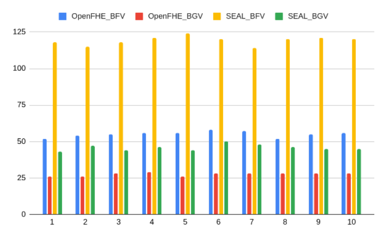
Visualization for Enhanced Comprehension

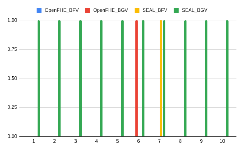
mult graph

X-axis : Inputx, Y-axis : overhead in milliseconds

Addition:

Input1Input2Input3OpenFHE_BFVOpenFHE_BGVSEAL_BFVSEAL_BGV
1230001
4560001
7890001
1011120001
1314150001
1617180101
1920210011
2223240001
2526270001
2829300001

Visualization for Enhanced Comprehension

addition graph

X-axis : Inputx, Y-axis : overhead in milliseconds

Comparing the overheads when FHE is not used

The GitHub repository also includes C programs that perform identical multiplication and addition operations on 64-bit integer values. The execution times are compared with FHE operations, revealing the overheads associated with FHE execution.

binaries/c_program.c

#include <stdio.h>
#include <stdlib.h>
#include <time.h>
#include <inttypes.h>

int main(int argc, char *argv[]) {
int64_t num1, num2, num3;


if (argc >= 4) {
num1 = strtoll(argv[1], NULL, 10);
num2 = strtoll(argv[2], NULL, 10);
num3 = strtoll(argv[3], NULL, 10);
} else {
printf("usage: ./c_program <num1> <num2> <num3> \n");
return 1;
}


int64_t add, mul;
clock_t start, end;
double add_time, mul_time;


start = clock();
add = num1 + num2 + num3;
end = clock();

add_time = ((double) (end - start)) / CLOCKS_PER_SEC * 1000; //time in milliseconds.


// Perform multiplication
start = clock();
mul = num1 * num2 * num3;
end = clock();
mul_time = ((double) (end - start)) / CLOCKS_PER_SEC * 1000; //time in milliseconds


// Output results
printf("mul_time: %lf add_time%lf\n", mul_time, add_time);

return 0;
}

Multiplication:

Input1Input2Input3non_FHEOpenFHE_BFVOpenFHE_BGVSEAL_BFVSEAL_BGV
1230.0009522611843
4560.001542611547
7890.001552811844
1011120.0009562912146
1314150.001562612444
1617180.0017582812050
1920210.0005572811448
2223240.0003522812046
2526270.0006552812145
2829300.0011562812045

Average Overheads:

Overheads (ms)non-FHEOpenFHE_BFVOpenFHE_BGVSEAL_BFVSEAL_BGV
Multiplication0.000955.099127.4991119.099145.7991

Addition:

Input1Input2Input3non_FHEOpenFHE_BFVOpenFHE_BGVSEAL_BFVSEAL_BGV
1230.00140001
4560.00170001
7890.0010001
1011120.00120001
1314150.0010001
1617180.0090101
1920210.00090011
2223240.00080001
2526270.00080001
2829300.00140001

Average Overheads:

Overheads (ms)non-FHEOpenFHE_BFVOpenFHE_BGVSEAL_BFVSEAL_BGV
Addition0.001920.0019200.10.1

Conclusion

Our analysis brings forth a compelling narrative. OpenFHE demonstrates superior implementation of FHE schemes, with OpenFHE_BGV emerging as the top performer, closely followed by OpenFHE_BFV. SEAL, while robust, exhibits higher runtimes compared to OpenFHE, suggesting that OpenFHE's implementation is more efficient.

Explore Further

To delve deeper into the world of homomorphic encryption and contribute to its advancements, consider exploring the GitHub repositories for OpenFHE and SEAL:

Download the respective binaries from the library repositories and engage in the evolving landscape of homomorphic encryption.

This exploration not only enhances our understanding of FHE but also contributes valuable insights to the ongoing development of secure and privacy-preserving computational technologies.

Appendix

This section provides details on the build process for two libraries. The instructions are presented to facilitate independent experimentation with Fully Homomorphic Encryption (FHE) implementations.

Prerequisites

To execute this project, ensure that the following dependencies are installed:

  • CMake
  • G++
  • GMP
  • Clang

OpenFHE

Navigate to the openfhe directory and follow these steps to set up the project:

mkdir build
cd build
cmake ..
make
make install
make testall

After modifying the code, compile test programs using the following commands:

make added_bgv
make added_bfv

To execute the examples, run the binaries as follows:

bin/examples/pke/added_bgv
bin/examples/pke/added_bfv

Additionally, new files created will be automatically linked during the make process.

SEAL

Set up this library with the following instructions:

cmake -S . -B build -DSEAL_BUILD_EXAMPLES=ON
cmake --build build
sudo cmake --install build

To run the compiled work, locate the binary at build/bin/sealexamples.

· 5 min read
Abid Arcot

Background: Understanding Physical Unclonable Functions (PUFs)

What are PUFs?

Physical Unclonable Functions (PUFs) are hardware-based security primitives that leverage the inherent manufacturing variations present in semiconductor devices. These variations, often microscopic and uncontrollable during fabrication, result in unique physical fingerprints for each device. PUFs exploit these variations to generate responses that are practically impossible to replicate, providing a reliable means of device authentication.

Importance in Hardware Security

PUFs play a crucial role in enhancing hardware security. Unlike traditional cryptographic methods that rely on stored secret keys, PUFs derive their security from the physical characteristics of the device. This makes PUFs resistant to various attacks, including invasive attacks attempting to clone or tamper with the device.

Applications of PUFs

  • Device Authentication: PUFs can be used to authenticate electronic devices by generating unique identifiers based on their physical characteristics.
  • Secure Key Generation: PUFs serve as a source of entropy for generating cryptographic keys, ensuring a high level of randomness and security.
  • Anti-Counterfeiting: PUFs help combat counterfeiting by providing a reliable way to verify the authenticity of electronic components.

In the subsequent sections, we will delve into the implementation details of Arbiter PUF and Ring Oscillator (RO) PUF, highlighting their design principles, testing methodologies, and achieved results.

Introduction

In the realm of hardware security and trust, the implementation of Physical Unclonable Functions (PUFs) stands as a formidable solution. This blog explores the design and implementation of two distinct PUF variants: Arbiter PUF and Ring Oscillator (RO) PUF. The source code and project details can be found on GitHub.

Arbiter PUF: Harnessing Delay Differences

Design Overview

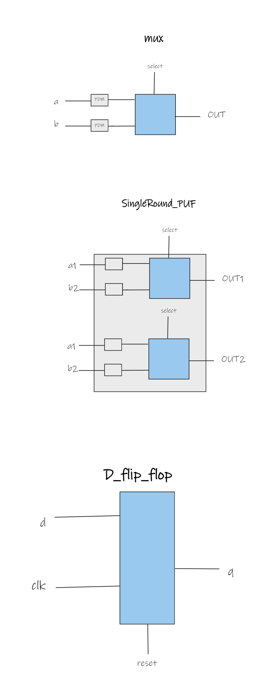
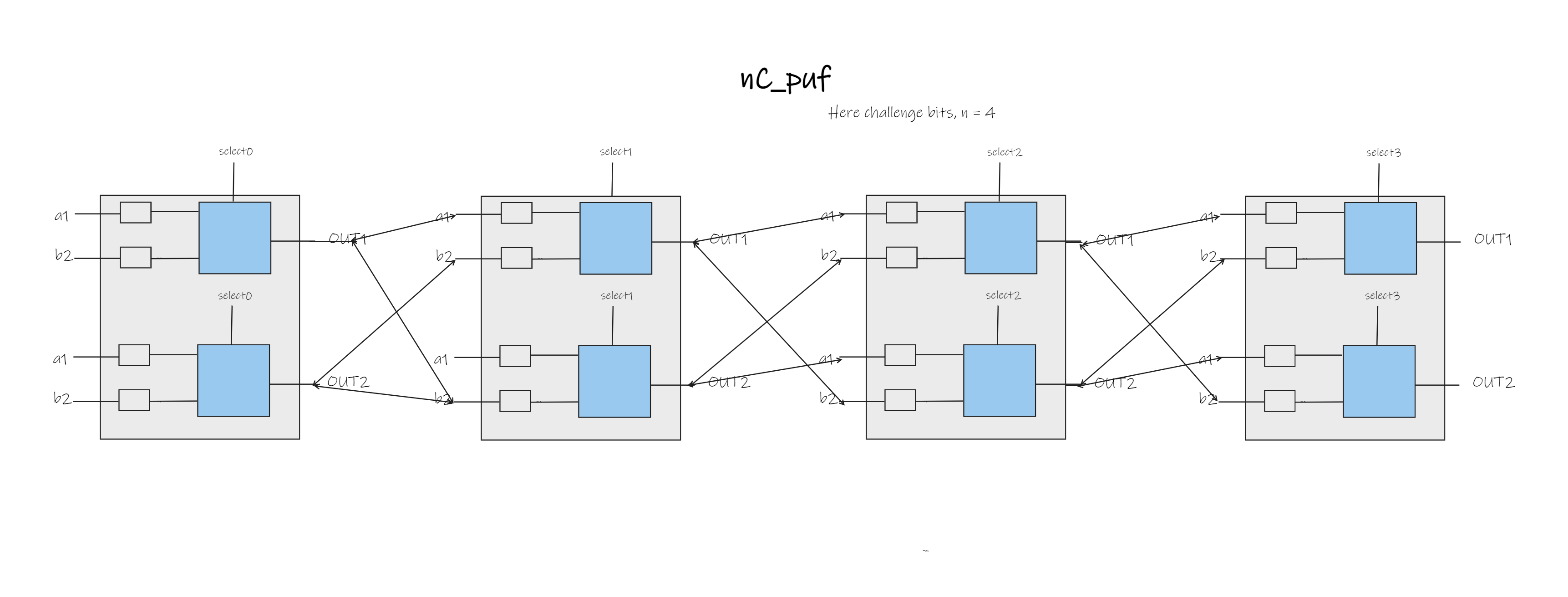
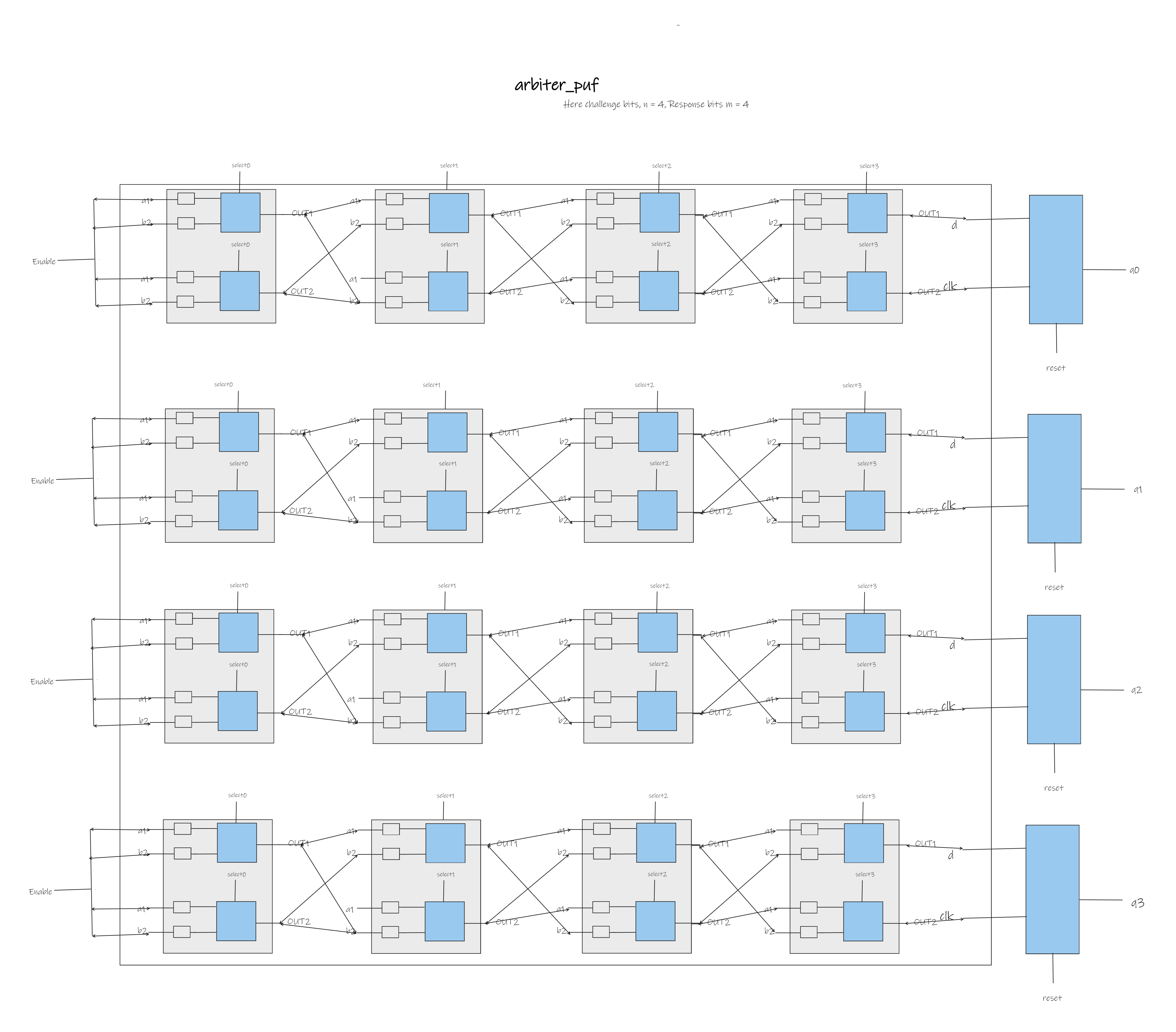
The Arbiter PUF relies on delay differences in multiplexers to generate unique responses based on challenge bits. Leveraging Verilog and ModelSim, we crafted a robust PUF architecture capable of handling a 4-bit challenge with 32-bit responses.

Implementation Details

To simulate the Arbiter PUF, we utilized the provided mux module with varying propagation delays. The 4-bit delay values for each multiplexer were parameterized using the DELAY parameter. The resulting PUF demonstrated an impressive single-chip Hamming distance of 49.10%, affirming its high-quality output.

Sub-Module Hierarchy and Design Decisions

Our design incorporated additional modules for a single response bit and a single round of the Arbiter PUF. The sub-module hierarchy was carefully crafted for modularity and scalability. The report details the design decisions made during the implementation.

components

single-response-puf

arbiter-puf

Verification and Testing

Ensuring the reliability of our PUF, we developed a comprehensive test bench for every module. The ModelSim GUI proved instrumental in observing signal waveforms and validating the functionality of the Arbiter PUF. The following table represents challenge-response pairs generated from random dealy parameter bits.

ChallengeResponse
000011010110000010111010110011001011
000111011110001010010111110111011011
001001111111101000000101101101010010
001101110111010001011110101001010010
010000110101001001000101001101010000
010110110101000101001101001101010100
011011110100000001111011010101010001
011111110000000001000011110101010001
100000110001100101000101001100110100
100110100101000101111101001110110100
101010000000000111111011010110110101
101111011000000101110011010110110101
110011001100010010111010110010101011
110111011000100010110111110110101011
111000011111111110010101101110110010
111100000111010110011110101010100110

The resulting PUF demonstrated an impressive single-chip Hamming distance of 49.10%, affirming its high-quality output.

Ring Oscillator PUF: Unleashing FPGA Potential

RO PUF Architecture

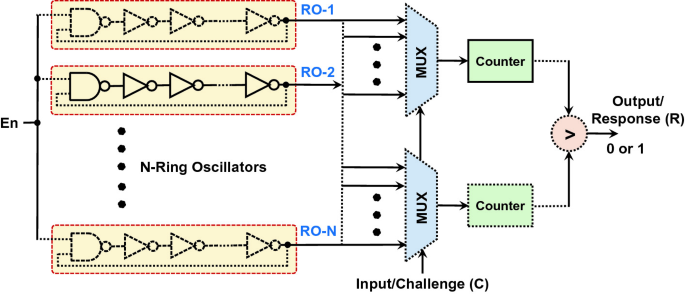
Shifting focus to the RO PUF, our implementation targeted a Cyclone V GX FPGA. This variant employed multiple Ring Oscillators, each with unique frequencies due to fabrication variations. Challenge-Response Pairs (CRPs) were generated by racing counters using different RO outputs as clocks. We implemented RO PUF capable of producing 8-bit Challenge - 4-bit Response pairs. For a given 8-bit challenge - 1-bit Response PUF as shown below where N=16, 4 MSB from 8-bit challenge is used to select the ring oscillator for first MUX and the remaining 4 LSB for second MUX.

ro-puf

2*log2(N)-bit Challenge - 1-bit Response RO PUF

Synthesis and FPGA Integration

We utilized Quartus Prime to synthesize the Verilog design into an FPGA bit-stream. The Chip Planner tool facilitated the careful placement of RO modules within a single LAB Cell, minimizing propagation delays and ensuring optimal performance.

Results and Quality Assessment

The RO PUF exhibited a single-chip Hamming distance of 41.30% for 8-bit Challenge - 4-bit Response pairs, showcasing its robustness, while the utilizing 192 ALMS. The following table represents challenge-response pairs generated from FPGA.

ChallengeFPGA Response
000000001111
100010010101
011100111010
000011010011
111001010111
001100010101
011001101111
110001100111
110010001110
100001111010
000000111010
111101110101
100000010101
101110111111
000000010010
101001100001
111010111111
000101100011
100111111000
010000000101
001111000101
001011111010
011111001010
010101011111

Conclusion

This technical blog provides a comprehensive insight into the implementation of Arbiter PUF and RO PUF. The GitHub repository contains the complete source code and project files for further exploration. The achieved Hamming distances underscore the effectiveness of these PUF variants in generating unique and secure responses.

For detailed code snippets, project files, and a deeper dive into the implementation, visit our GitHub repository.

· 3 min read
Abid Arcot

Introduction

In the fast-evolving landscape of mobile computing, the convergence of edge devices and advanced image classification techniques holds immense promise. This blog documents a compelling project undertaken within the purview of CSE 535 Mobile Computing, spotlighting the seamless integration of server-side processes for image classification on edge devices. Through a meticulous blend of Android application development, convolutional neural networks (CNNs) and Server integration, this endeavor illuminates the transformative potential of server integration in enhancing mobile computing capabilities.

Project Overview

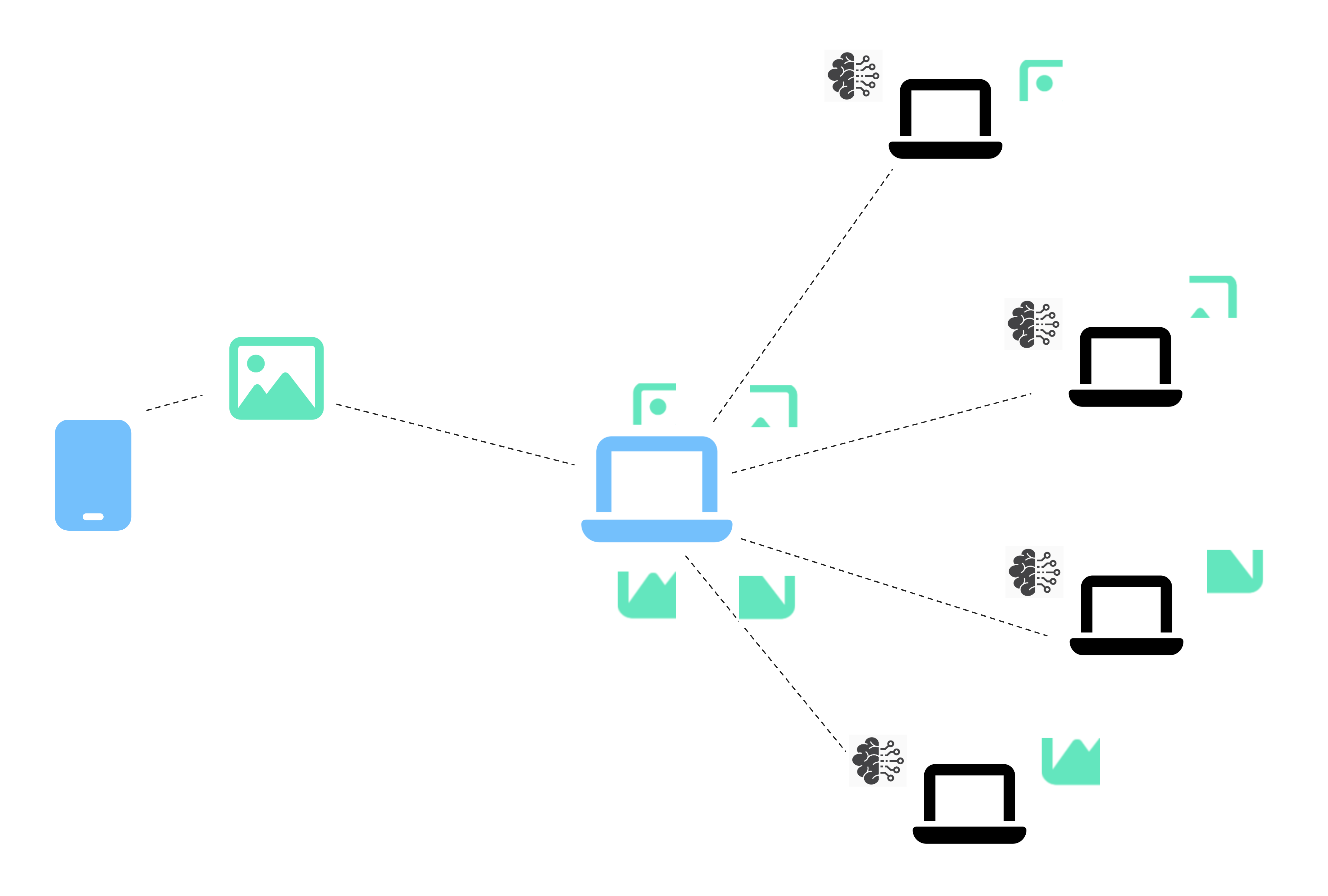
This project aims to utilize an Android application to divide captured images into parts for classification on edges devices like mobiles, laptops etc. Leveraging a CNN model trained on the MNIST dataset, the goal is to accurately categorize handwritten digits and organize them into respective folders based on their content.

Overview-img

Implementation Details

Building the Android Application

  • MainActivity.java and ImageCaptureActivity.java formed the backbone of the application, augmented by XML layout files to craft a seamless user interface.
  • Image division into four parts, facilitated by bitmap manipulation, enabled efficient processing and distribution to client edge devices.
main-page
capture-page
addition-page
veiw-1, veiw-2, view-3

Dividing the Image

  • Employing bitmap division techniques, captured images were sliced into manageable components for parallel processing.
  • Each edge device, acting as a server, received a distinct image part for classification, optimizing resource utilization and minimizing latency.
partion-preview
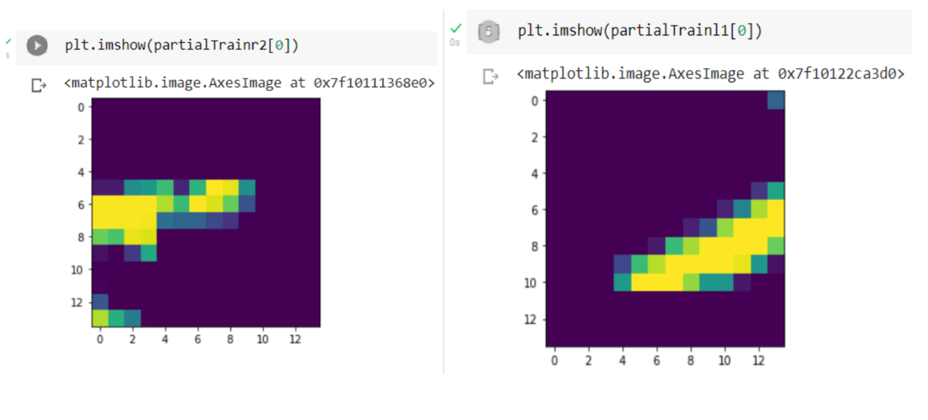
Image samples after divison

Deep Learning Model

  • A robust CNN model, with an accuracy of 80.34% on the MNIST dataset, has been employed for the image classification efforts.
  • We hae used the CNN model with 1 input layer, 2 hidden layers and 1 output layer using activation function relu for hidden layers and softmax for output layer.

Server Integration

  • Flask servers, equipped with CNN models, awaited image parts for classification, seamlessly interfacing with the main mobile application.
  • Retrofit and OKHTTP3 libraries facilitated smooth communication between the mobile and server edge devices, ensuring swift data transmission and response retrieval.
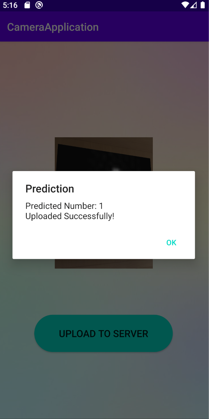
  • Upon receiving predictions, the mobile application intelligently stored original images in designated folders based on classification confidence, exemplifying the project's end-to-end integration process.
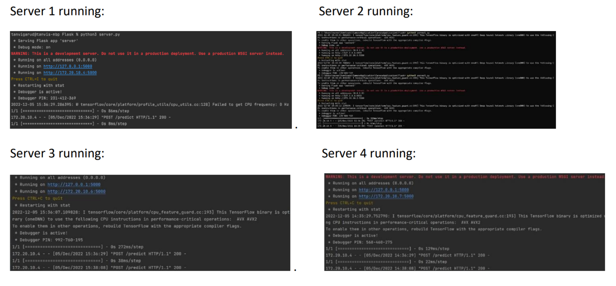
running-servers
Servers running on different edge devices connected over local network

Results

The following are the key aspects of the project that we have implemented and achieved:

  • Launching and navigation through the Android application's user interface.
  • Capturing images using the device's camera and initiating the image classification process.
  • Seamless communication between the mobile application and server edge devices.
  • Real-time classification of handwritten digits and organization into respective folders based on classification results received from offloaded servers.

Conclusion

In summary, the integration of server-side processes for image classification on edge devices represents a paradigm shift in mobile computing. By harnessing the collaborative power of Android application development, deep learning, and server integration, this project underscores the transformative potential of mobile computing in real-world applications.

Source Code

Explore the source code of this project on GitHub: GitHub Repository